Understanding the Filter Function in Excel

 

Table of Contents Introduction Syntax of the Filter Function Uses of the Filter Function 10 Examples Using the Filter Function Conclusion

 

Introduction

The FILTER function in Excel is a powerful tool that allows users to extract specific data from a range based on defined criteria. This function simplifies the process of analyzing and manipulating large datasets by enabling you to display only the information that meets certain conditions. In this article, we will explore the FILTER function in detail, including its syntax, uses, and along with ten examples using student performance data. Whether you're a beginner or looking to enhance your Excel skills, this guide will take you from novice to expert in no time!

Syntax of the Filter Function

The syntax of the FILTER function is straightforward. Here’s how it looks:

=FILTER(array, include, [if_empty])

Parameters:

• array: This is the range of data you want to filter. It includes all the columns you wish to extract.
• include: This parameter specifies the condition(s) that must be met for the data to be included in the result. It should return TRUE or FALSE values.
• [if_empty]: This optional parameter allows you to specify a value to return if no data meets the criteria.

Uses of the Filter Function

The FILTER function can be used for various tasks, such as:

• Displaying subsets of data based on specific conditions.
• Analyzing student performance by grade, score, or attendance.
• Creating dynamic reports that update automatically as data changes.

With the basic understanding of the FILTER function, let's explore practical examples using a dataset containing student information.

10 Examples Using the Filter Function

Below is a dataset of student performance:

1. Filter by Grade

To show only the students who are in grade 10, we can use the FILTER function. This function allows us to extract rows that meet specific conditions. The formula to filter for grade 10 is:

=FILTER(A2:O11, D2:D11=10)

In this formula, A2:O11 represents the range of data we want to filter, and D2:D11=10 is the condition specifying that we only want students in grade 10. When you enter this formula, Excel will return all rows from the dataset where the grade is 10, making it easy to focus on these students.

2. Filter by City

If you want to get a list of students from a specific city, say City A, you would use the following formula:

=FILTER(A2:O11, H2:H11="City A")

Here, H2:H11="City A" is the condition that filters for students living in City A. This formula extracts all relevant rows, allowing you to analyze or report specifically on students from that city.

3. Filter by Score Above 80

To find students who scored above 80, you can apply the FILTER function like this:

=FILTER(A2:O11, F2:F11>80)

In this case, F2:F11>80 checks the score column to see which students have scores greater than 80. The result will be a list of all students who achieved this score, helping you identify high achievers.

4. Combine FILTER with COUNTA

If you want to count how many students scored above 80, you can combine FILTER with COUNTA like this:

=COUNTA(FILTER(A2:A11, F2:F11>80))

This formula first filters the student list to find those with scores above 80 and then counts how many entries are in that filtered list. The result will give you the total number of students who excelled.

5. Filter by Scholarship Status

To list students who received scholarships, use the following formula:

=FILTER(A2:O11, N2:N11="Yes")

In this example, N2:N11="Yes" is the condition that filters for students with a scholarship status of "Yes." The output will display all the students who have received scholarships, making it easy to view this group.

6. Filter by Enrollment Date

If you're interested in listing students who enrolled after January 1, 2021, the formula would be:

=FILTER(A2:O11, K2:K11>DATE(2021,1,1))

Here, K2:K11>DATE(2021,1,1) filters for enrollment dates that are after the specified date. This can help you analyze the most recent enrollments in your dataset.

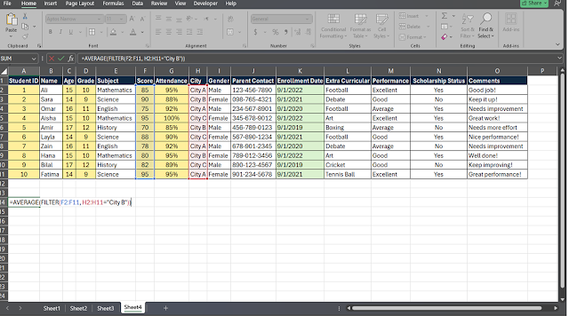
7. Combine FILTER with AVERAGE

To calculate the average score of students from City B, you can combine FILTER with the AVERAGE function:

=AVERAGE(FILTER(F2:F11, H2:H11="City B"))

In this formula, FILTER retrieves scores of students from City B, and AVERAGE computes the average of these scores. This provides insights into the performance of students specifically from City B.

8. Filter for Recent Enrollments

To show students who enrolled in the last year, you can use:

=FILTER(A2:O11, K2:K11>=DATE(YEAR(TODAY())-1,1,1))

This formula checks the enrollment date column to find students who enrolled on or after January 1 of the previous year. It's useful for tracking new enrollments within a specific timeframe.

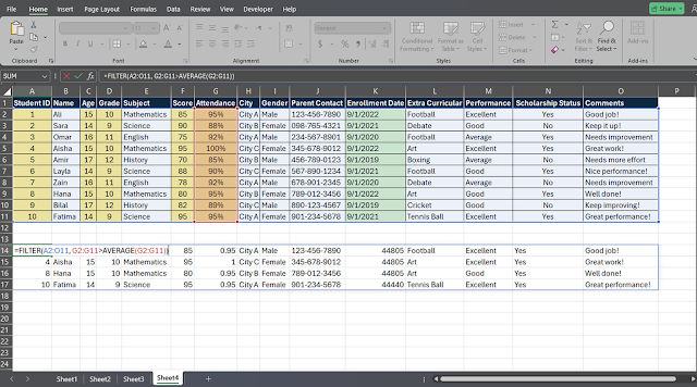
9. Filter for Above Average Attendance

To find students with above-average attendance, use this formula:

=FILTER(A2:O11, G2:G11>AVERAGE(G2:G11))

This formula first calculates the average attendance using AVERAGE(G2:G11) and then filters the list to find students with attendance greater than this average. This helps identify students who are more consistently present.

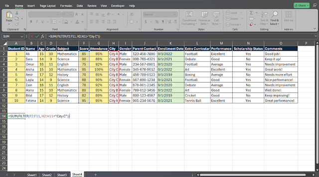
10. Filter and Aggregate Score

To calculate the total score of students in City C, you would use:

=SUM(FILTER(F2:F11, H2:H11="City C"))

Here, FILTER extracts the scores of students from City C, and SUM adds them together. The result gives you the total score for all students in that city, allowing for quick performance assessments.

Conclusion

The FILTER function is a versatile tool that allows you to manipulate and analyze data effectively in Excel. By learning how to use this function with practical examples, you can quickly become proficient in handling datasets, whether for academic, business, or personal purposes. With the skills gained from this guide, you can efficiently extract and analyze data to make informed decisions. Start practicing the examples provided and explore further possibilities with the FILTER function!

Click here to download template